Retrieving snow and ice albedo from Landsat data
Source:vignettes/albedo_retrieval_landsat.Rmd
albedo_retrieval_landsat.RmdThis vignette shows how to use Landsat surface reflectance,
topographic data, and glacier outlines to retrieve snow and ice albedo
at the Athabasca Glacier in Canada. We provide the input datasets for 16
August 2020 and guide the user through the processing steps implemented
in SatRbedo. It is assumed that users have basic knowledge
of geographic information systems, satellite remote sensing, and
accessing Earth Observation data.
Load the required packages
First, we load the SatRbedo and terra
packages. The latter is used for spatial data manipulation,
visualization, and analysis.
Input data
Landsat surface reflectance (Landsat Collection 2 Level-2) and topographic (e.g., SRTM) data for the area of interest can be downloaded from the USGS EarthExplorer. Glacier outlines are available on the GLIMS website.
The SatRbedo package provides functions to calculate
albedo using two (green and near-infrared), four (blue, green, red, and
near-infrared), and five (blue, red, near-infrared, shortwave-infrared
1, and shortwave-infrared 2) spectral bands. These functions also
require the solar and view angles. To generate these angles, the Landsat
Angles Creation Tools can be used.
After downloading the necessary input data, reproject the digital
elevation model (DEM) grid and the glacier outline shapefile to
Landsat’s coordinate system, then resample the DEM to 30 m spatial
resolution. Select scenes with minimal cloud coverage and crop the DEM,
surface reflectance, and angle bands to the area of interest. These
tasks can be performed using the preproc() function and the
terra package.
Below, we provide the necessary input data to run the
SatRbedo functions for the area of interest:
# Load the Landsat surface reflectance bands
blue_SR <- system.file("extdata/athabasca_2020229_B02_L30.tif", package = "SatRbedo") # blue band surface reflectance (Landsat band 2)
green_SR <- system.file("extdata/athabasca_2020229_B03_L30.tif", package = "SatRbedo") # green band surface reflectance (Landsat band 3)
red_SR <- system.file("extdata/athabasca_2020229_B04_L30.tif", package = "SatRbedo") # red band surface reflectance (Landsat band 4)
NIR_SR <- system.file("extdata/athabasca_2020229_B05_L30.tif", package = "SatRbedo") # near-infrared band surface reflectance (Landsat band 5)
SWIR1_SR <- system.file("extdata/athabasca_2020229_B06_L30.tif", package = "SatRbedo") # shortwave-infrared band 1 surface reflectance (Landsat band 6)
SWIR2_SR <- system.file("extdata/athabasca_2020229_B07_L30.tif", package = "SatRbedo") # shortwave-infrared band 2 surface reflectance (Landsat band 7)

# Load the DEM and the glacier outline
dem <- system.file("extdata/athabasca_dem.tif", package = "SatRbedo")
outline <- system.file("extdata/athabasca_outline.shp", package = "SatRbedo")

# Transform the raster data to SpatRaster and the glacier outline to SpatVector
dem <- terra::rast(dem)
glacier_mask <- terra::vect(outline)
blue <- terra::rast(blue_SR)
green <- terra::rast(green_SR)
red <- terra::rast(red_SR)
nir <- terra::rast(NIR_SR)
swir1 <- terra::rast(SWIR1_SR)
swir2 <- terra::rast(SWIR2_SR)
Topographic correction
The topographic correction compensates for differences in solar
illumination caused by elevation, slope, aspect, and the obstruction of
surrounding terrain. The topographic correction methods implemented in
SatRbedo require the removal of terrain shadow effects,
including self and cast shadows. This can be achieved with the
shadow_removal() function:
SAA <- 154.6 # solar azimuth angle
SZA <- 40.8 # solar zenith angle
msk <- shadow_removal(dem, SZA, SAA, mask = TRUE) # Shadow mask

# Remove shadowed pixels
blue_masked <- blue * msk
green_masked <- green * msk
red_masked <- red * msk
nir_masked <- nir * msk
swir1_masked <- swir1 * msk
swir2_masked <- swir2 * msk
Then, the topographic correction is carried out using the
topo_corr() function:
# Topographic correction using method = "tanrotation"
blue_corr <- topo_corr(blue_masked, dem, SAA, SZA, method = "tanrotation")
green_corr <- topo_corr(green_masked, dem, SAA, SZA, method = "tanrotation")
red_corr <- topo_corr(red_masked, dem, SAA, SZA, method = "tanrotation")
nir_corr <- topo_corr(nir_masked, dem, SAA, SZA, method = "tanrotation")
swir1_corr <- topo_corr(swir1_masked, dem, SAA, SZA, method = "tanrotation")
swir2_corr <- topo_corr(swir2_masked, dem, SAA, SZA, method = "tanrotation")

# Topographic correction using method = "ccorrection"
blue_corr_c <- topo_corr(blue_masked, dem, SAA, SZA, method = "ccorrection", IC_min = 0.3)
green_corr_c <- topo_corr(green_masked, dem, SAA, SZA, method = "ccorrection", IC_min = 0.3)
red_corr_c <- topo_corr(red_masked, dem, SAA, SZA, method = "ccorrection", IC_min = 0.3)
nir_corr_c <- topo_corr(nir_masked, dem, SAA, SZA, method = "ccorrection", IC_min = 0.3)
swir1_corr_c <- topo_corr(swir1_masked, dem, SAA, SZA, method = "ccorrection", IC_min = 0.3)
swir2_corr_c <- topo_corr(swir2_masked, dem, SAA, SZA, method = "ccorrection", IC_min = 0.3)
The first method (method = “tanrotation”) is preferred because it does not overcorrect surface reflectance in low-illumination regions.
Discrimination of snow and ice pixels
The algorithm for distinguishing snow from ice surfaces uses the green and near-infrared surface reflectance bands. It is applied to all pixels within the glacier mask.
green_crop <- terra::crop(green, glacier_mask, mask = TRUE)
nir_crop <- terra::crop(nir, glacier_mask, mask = TRUE)
surf_type <- snow_or_ice(green_crop, nir_crop)
thres <- surf_type$th
plot(surf_type$NDSII > thres, type = "classes",
  col = c("#FFFFC8", "#00407F"), levels = c("snow", "ice"))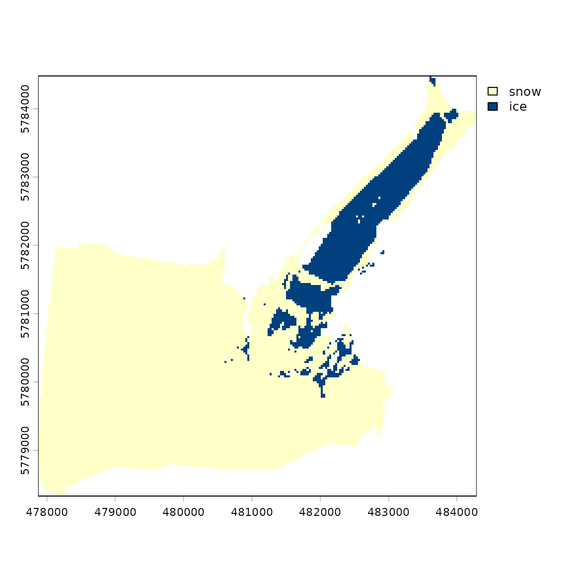
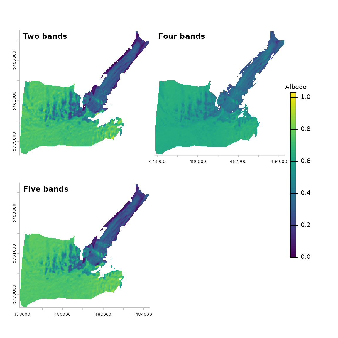
Estimation of broadband albedo after anisotropic correction
Finally, broadband albedo can be calculated using three different
methods through the albedo_sat() function.
SAA <- 154.6 # solar azimuth angle
SZA <- 40.8 # solar zenith angle
VAA <- 266.3 # view azimuth angle
VZA <- 4.1 # view zenith angle

# Use the glacier mask to crop the DEM and the topographically-corrected bands
dem_crop <- terra::crop(dem, glacier_mask, mask = TRUE)
slope <- terra::terrain(dem_crop, v = "slope", neighbors = 4, unit = "degrees")
aspect <- terra::terrain(dem_crop, v = "aspect", neighbors = 4, unit = "degrees")
blue_crop <- terra::crop(blue_corr$bands[[2]], glacier_mask, mask = TRUE)
green_crop <- terra::crop(green_corr$bands[[2]], glacier_mask, mask = TRUE)
red_crop <- terra::crop(red_corr$bands[[2]], glacier_mask, mask = TRUE)
nir_crop <- terra::crop(nir_corr$bands[[2]], glacier_mask, mask = TRUE)
swir1_crop <- terra::crop(swir1_corr$bands[[2]], glacier_mask, mask = TRUE)
swir2_crop <- terra::crop(swir2_corr$bands[[2]], glacier_mask, mask = TRUE)

albedo_two <- albedo_sat(
  SAA, SZA, VAA, VZA,
  slope, aspect, method = "twobands",
  green = green_crop, NIR = nir_crop, th = thres
)

albedo_four <- albedo_sat(
  method = "fourbands",
  blue = blue_crop, green = green_crop, red = red_crop, NIR = nir_crop
)

albedo_five <- albedo_sat(
  SAA, SZA, VAA, VZA,
  slope, aspect, method = "fivebands",
  blue = blue_crop, green = green_crop, red = red_crop,
  NIR = nir_crop, SWIR1 = swir1_crop, SWIR2 = swir2_crop, th = thres
)

# Plot the results
albedo <- c(albedo_two[[3]], albedo_four[[5]], albedo_five[[6]])
names(albedo) <- c("Two bands", "Four bands", "Five bands")
panel(albedo, plg = list(title = "Albedo"))