This document aims to introduce users to the basic functionality of
SatRbedo. The example demonstrates how to use the package
to compute snow and ice albedo at the Athabasca Glacier in Canada from
five spectral bands. It utilises Sentinel-2 surface reflectance data
measured on 9 September 2020.
First, we load the SatRbedo and terra
packages. The latter is used for spatial data manipulation,
visualization, and analysis.
The process for generating satellite albedo retrievals involves five steps:
Step 1: Load the data for the area of interest
# Load Sentinel-2 surface reflectance data
# Note: each spectral band was previously cut out to the extent of the area of interest and renamed
blue_SR <- system.file("extdata/athabasca_2020253_B02_S30.tif", package = "SatRbedo") # blue band surface reflectance (Sentinel-2 band 2)
green_SR <- system.file("extdata/athabasca_2020253_B03_S30.tif", package = "SatRbedo") # green band surface reflectance (Sentinel-2 band 3)
red_SR <- system.file("extdata/athabasca_2020253_B04_S30.tif", package = "SatRbedo") # red band surface reflectance (Sentinel-2 band 4)
NIR_SR <- system.file("extdata/athabasca_2020253_B8A_S30.tif", package = "SatRbedo") # near-infrared band surface reflectance (Sentinel-2 band 8A)
SWIR1_SR <- system.file("extdata/athabasca_2020253_B11_S30.tif", package = "SatRbedo") # shortwave-infrared band 1 surface reflectance (Sentinel-2 band 11)
SWIR2_SR <- system.file("extdata/athabasca_2020253_B12_S30.tif", package = "SatRbedo") # shortwave-infrared band 2 surface reflectance (Sentinel-2 band 12)

# Load the DEM and the outline
# Note: the DEM was re-projected to the extent of the area of interest and
# resampled to a 30 m spatial resolution
dem <- system.file("extdata/athabasca_dem.tif", package = "SatRbedo")
outline <- system.file("extdata/athabasca_outline.shp", package = "SatRbedo")
Step 2: Data pre-processing
# Transform the raster data to SpatRaster and the glacier outline to SpatVector
dem <- terra::rast(dem)
glacier_mask <- terra::vect(outline)
AOI <- terra::ext(477870, 484320, 5778330, 5784480) # Area of interest
blue <- preproc(grd = blue_SR, outline = AOI)
green <- preproc(grd = green_SR, outline = AOI)
red <- preproc(grd = red_SR, outline = AOI)
nir <- preproc(grd = NIR_SR, outline = AOI)
swir1 <- preproc(grd = SWIR1_SR, outline = AOI)
swir2 <- preproc(grd = SWIR2_SR, outline = AOI)
Step 3: Topographic correction
SAA <- 167.8 # solar azimuth angle
SZA <- 47.8 # solar zenith angle

# Detect and remove topographic shadows
msk <- shadow_removal(dem, SZA, SAA, mask = TRUE) # Shadow mask
blue_masked <- blue * msk
green_masked <- green * msk
red_masked <- red * msk
nir_masked <- nir * msk
swir1_masked <- swir1 * msk
swir2_masked <- swir2 * msk

# Perform the topographic correction
blue_corr <- topo_corr(blue_masked, dem, SAA, SZA)
green_corr <- topo_corr(green_masked, dem, SAA, SZA)
red_corr <- topo_corr(red_masked, dem, SAA, SZA)
nir_corr <- topo_corr(nir_masked, dem, SAA, SZA)
swir1_corr <- topo_corr(swir1_masked, dem, SAA, SZA)
swir2_corr <- topo_corr(swir2_masked, dem, SAA, SZA)
Step 4: Discrimination of snow and ice pixels
# Use the glacier mask to crop the green and NIR spectral bands
green_crop <- terra::crop(green, glacier_mask, mask = TRUE)
nir_crop <- terra::crop(nir, glacier_mask, mask = TRUE)

# Calculate the threshold used to discriminate between snow and ice
threshold <- snow_or_ice(green_crop, nir_crop)$th
Step 5: Estimation of broadband albedo after anisotropic correction
SAA <- 167.8 # solar azimuth angle
SZA <- 47.8 # solar zenith angle
VAA <- 277.6 # view azimuth angle
VZA <- 8.4 # view zenith angle

# In this example, we will calculate broadband albedo using five spectral bands
# Use the glacier mask to crop the DEM and the topographically-corrected bands
dem_crop <- terra::crop(dem, glacier_mask, mask = TRUE)
slope <- terra::terrain(dem_crop, v = "slope", neighbors = 4, unit = "degrees")
aspect <- terra::terrain(dem_crop, v = "aspect", neighbors = 4, unit = "degrees")
blue_crop <- terra::crop(blue_corr$bands[[2]], glacier_mask, mask = TRUE)
green_crop <- terra::crop(green_corr$bands[[2]], glacier_mask, mask = TRUE)
red_crop <- terra::crop(red_corr$bands[[2]], glacier_mask, mask = TRUE)
nir_crop <- terra::crop(nir_corr$bands[[2]], glacier_mask, mask = TRUE)
swir1_crop <- terra::crop(swir1_corr$bands[[2]], glacier_mask, mask = TRUE)
swir2_crop <- terra::crop(swir2_corr$bands[[2]], glacier_mask, mask = TRUE)

broadband_albedo <- albedo_sat(
  SAA, SZA, VAA, VZA,
  slope, aspect, method = "fivebands",
  blue = blue_crop, green = green_crop, red = red_crop,
  NIR = nir_crop, SWIR1 = swir1_crop, SWIR2 = swir2_crop,
  th = threshold
)

# Plot the results
plot(broadband_albedo[[6]], plg = list(title = "Albedo"))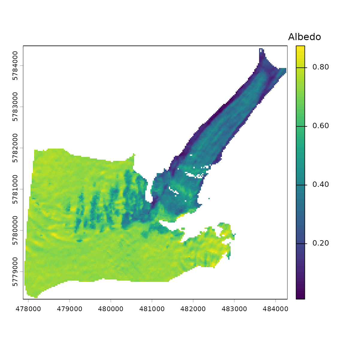
Where to go next?
You can check the function documentation here.
A more elaborate example using Landsat data can be found in
vignette("albedo_retrieval_landsat").